Z-transform

From Wikipedia, the free encyclopedia

Jump to: navigation, search

In mathematics and signal processing, the Z-transform converts a discrete time-domain signal, which is a sequence of real or complex numbers, into a complex frequency-domain representation.
It can be considered as a discrete-time equivalent of the Laplace transform. This similarity is explored in the theory of time scale calculus.

History

The basic idea now known as the Z-transform was known to Laplace, and re-introduced in 1947 by W. Hurewicz as a tractable way to solve linear, constant-coefficient difference equations.^[1] It was later dubbed "the z-transform" by Ragazzini and Zadeh in the sampled-data control group at Columbia University in 1952.^[2]^[3]
The modified or advanced Z-transform was later developed and popularized by E. I. Jury.^[4]^[5]
The idea contained within the Z-transform is also known in mathematical literature as the method of generating functions which can be traced back as early as 1730 when it was introduced by de Moivre in conjunction with probability theory.^[6] From a mathematical view the Z-transform can also be viewed as a Laurent series where one views the sequence of numbers under consideration as the (Laurent) expansion of an analytic function.

Definition

The Z-transform, like many integral transforms, can be defined as either a one-sided or two-sided transform.

Bilateral Z-transform

The bilateral or two-sided Z-transform of a discrete-time signal x[n] is the formal power series X(z) defined as

$X(z) = \mathcal{Z}\{x[n]\} = \sum_{n=-\infty}^{\infty} x[n] z^{-n}$

where n is an integer and z is, in general, a complex number:

$z = A e^{j\phi} = A(\cos{\phi}+j\sin{\phi})\,$

where A is the magnitude of z, j is the imaginary unit, and $\phi$ is the complex argument (also referred to as angle or phase) in radians.

Unilateral Z-transform

Alternatively, in cases where x[n] is defined only for n ≥ 0, the single-sided or unilateral Z-transform is defined as

$X(z) = \mathcal{Z}\{x[n]\} = \sum_{n=0}^{\infty} x[n] z^{-n}. \$

In signal processing, this definition can be used to evaluate the Z-transform of the unit impulse response of a discrete-time causal system.
An important example of the unilateral Z-transform is the probability-generating function, where the component $x[n]$ is the probability that a discrete random variable takes the value $n$ , and the function $X(z)$ is usually written as $X(s)$ , in terms of $s = z^{-1}$ . The properties of Z-transforms (below) have useful interpretations in the context of probability theory.

Geophysical definition

In geophysics, the usual definition for the Z-transform is a power series in z as opposed to $z^{-1}$ . This convention is used by Robinson and Treitel and by Kanasewich.^{[citation needed]} The geophysical definition is

$X(z) = \mathcal{Z}\{x[n]\} = \sum_{n} x[n] z^{n}. \$

The two definitions are equivalent; however, the difference results in a number of changes. For example, the location of zeros and poles move from inside the unit circle using one definition, to outside the unit circle using the other definition. Thus, care is required to note which definition is being used by a particular author.

Inverse Z-transform

The inverse Z-transform is

$x[n] = \mathcal{Z}^{-1} \{X(z) \}= \frac{1}{2 \pi j} \oint_{C} X(z) z^{n-1} dz \$

where $C \$ is a counterclockwise closed path encircling the origin and entirely in the region of convergence (ROC). In the case where the ROC is causal (see Example 2), this means the path $C \$ must encircle all of the poles of $X(z) \$ .
A special case of this contour integral occurs when $C \$ is the unit circle (and can be used when the ROC includes the unit circle which is always guaranteed when $X(z)\$ is stable, i.e. all the poles are within the unit circle). The inverse Z-transform simplifies to the inverse discrete-time Fourier transform:

$x[n] = \frac{1}{2 \pi} \int_{-\pi}^{+\pi} X(e^{j \omega}) e^{j \omega n} d \omega. \$

The Z-transform with a finite range of n and a finite number of uniformly-spaced z values can be computed efficiently via Bluestein's FFT algorithm. The discrete-time Fourier transform (DTFT) (not to be confused with the discrete Fourier transform (DFT)) is a special case of such a Z-transform obtained by restricting z to lie on the unit circle.

Region of convergence

The region of convergence (ROC) is the set of points in the complex plane for which the Z-transform summation converges.

$ROC = \left\{ z : \left|\sum_{n=-\infty}^{\infty}x[n]z^{-n}\right| < \infty \right\}$

Example 1 (no ROC)

Let $x[n] = 0.5^n\$ . Expanding $x[n]\$ on the interval $(-\infty, \infty)\$ it becomes

$x[n] = \{..., 0.5^{-3}, 0.5^{-2}, 0.5^{-1}, 1, 0.5, 0.5^2, 0.5^3, ...\} = \{..., 2^3, 2^2, 2, 1, 0.5, 0.5^2, 0.5^3, ...\}\ .$

Looking at the sum

$\sum_{n=-\infty}^{\infty}x[n]z^{-n} \rightarrow \infty\ .$

Therefore, there are no values of $z\$ that satisfy this condition.

Example 2 (causal ROC)

ROC shown in blue, the unit circle as a dotted grey circle (appears reddish to the eye) and the circle $\left|z\right| = 0.5$ is shown as a dashed black circle

Let $x[n] = 0.5^n u[n]\$ (where $u$ is the Heaviside step function). Expanding $x[n]\$ on the interval $(-\infty, \infty)\$ it becomes

$x[n] = \{..., 0, 0, 0, 1, 0.5, 0.5^2, 0.5^3, ...\}.\$

Looking at the sum

$\sum_{n=-\infty}^{\infty}x[n]z^{-n} = \sum_{n=0}^{\infty}0.5^nz^{-n} = \sum_{n=0}^{\infty}\left(\frac{0.5}{z}\right)^n = \frac{1}{1 - 0.5z^{-1}}.\$

The last equality arises from the infinite geometric series and the equality only holds if $\left|0.5 z^{-1}\right| < 1\$ which can be rewritten in terms of $z\$ as $\left|z\right| > 0.5\$ . Thus, the ROC is $\left|z\right| > 0.5\$ . In this case the ROC is the complex plane with a disc of radius 0.5 at the origin "punched out".

Example 3 (anticausal ROC)

ROC shown in blue, the unit circle as a dotted grey circle and the circle $\left|z\right| = 0.5$ is shown as a dashed black circle

Let $x[n] = -(0.5)^n u[-n-1]\$ (where $u$ is the Heaviside step function). Expanding $x[n]\$ on the interval $(-\infty, \infty)\$ it becomes

$x[n] = \{..., -(0.5)^{-3}, -(0.5)^{-2}, -(0.5)^{-1}, 0, 0, 0, 0, ...\}.\$

Looking at the sum

$\sum_{n=-\infty}^{\infty}x[n]z^{-n} = -\sum_{n=-\infty}^{-1}0.5^nz^{-n} = -\sum_{n=-\infty}^{-1}\left(\frac{z}{0.5}\right)^{-n}\$

$= -\sum_{m=1}^{\infty}\left(\frac{z}{0.5}\right)^{m} = -\frac{1}{1 - 0.5^{-1}z}.\$

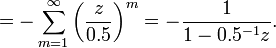
Using the infinite geometric series, again, the equality only holds if $\left|0.5^{-1}z\right| < 1\$ which can be rewritten in terms of $z\$ as $\left|z\right| < 0.5\$ . Thus, the ROC is $\left|z\right| < 0.5\$ . In this case the ROC is a disc centered at the origin and of radius 0.5.
What differentiates this example from the previous example is only the ROC. This is intentional to demonstrate that the transform result alone is insufficient.

Examples conclusion

Examples 2 & 3 clearly show that the Z-transform $X(z)\$ of $x[n]\$ is unique when and only when specifying the ROC. Creating the pole-zero plot for the causal and anticausal case show that the ROC for either case does not include the pole that is at 0.5. This extends to cases with multiple poles: the ROC will never contain poles.
In example 2, the causal system yields an ROC that includes $\left| z \right| = \infty\$ while the anticausal system in example 3 yields an ROC that includes $\left| z \right| = 0\$ .

ROC shown as a blue ring $0.5 < \left| z \right| < 0.75\$

In systems with multiple poles it is possible to have an ROC that includes neither $\left| z \right| = \infty\$ nor $\left| z \right| = 0\$ . The ROC creates a circular band. For example, $x[n] = 0.5^nu[n] - 0.75^nu[-n-1]\$ has poles at 0.5 and 0.75. The ROC will be $0.5 < \left| z \right| < 0.75\$ , which includes neither the origin nor infinity. Such a system is called a mixed-causality system as it contains a causal term $0.5^nu[n]\$ and an anticausal term $-(0.75)^nu[-n-1]\$ .
The stability of a system can also be determined by knowing the ROC alone. If the ROC contains the unit circle (i.e., $\left| z \right| = 1\$ ) then the system is stable. In the above systems the causal system (Example 2) is stable because $\left| z \right| > 0.5\$ contains the unit circle.
If you are provided a Z-transform of a system without an ROC (i.e., an ambiguous $x[n]\$ ) you can determine a unique $x[n]\$ provided you desire the following:

Stability
Causality

If you need stability then the ROC must contain the unit circle. If you need a causal system then the ROC must contain infinity and the system function will be a right-sided sequence. If you need an anticausal system then the ROC must contain the origin and the system function will be a left-sided sequence. If you need both, stability and causality, all the poles of the system function must be inside the unit circle.
The unique $x[n]\$ can then be found.

2 comments:

rajputJune 29, 2012 at 11:40 PM
Z-transform comes in mathematics and signal processing, the Z-transform converts a sequence of real or complex numbers into a complex frequency-domain representation.It can be considered as a discrete-time equivalent of the Laplace transform.
Critical Point

Programming + Errors

Thursday, May 17, 2012

Z- Transform

Z-transform

Contents

History

Definition

Bilateral Z-transform

Unilateral Z-transform

Geophysical definition

Inverse Z-transform

Region of convergence

Example 1 (no ROC)

Example 2 (causal ROC)

Example 3 (anticausal ROC)

Examples conclusion

2 comments:

Blog Archive